Why Is the On-Site PDA Value Alone Not Enough?

The value the PDA displays on site is a preliminary estimate, because it is computed from a simplified formula and assumes a single soil parameter for the whole pile.

During a PDA (dynamic load test), the instrument displays the bearing capacity immediately after every blow using a formula known as the Case Method. The advantage is fast results that can be used for decisions on site. The limitation is that it must assume a single soil parameter (damping factor) for the whole system. This value depends on the soil type and the tester's experience; different assumptions give different capacities.

CAPWAP overcomes this limitation by letting the measured data decide instead of assuming a single value. The model divides the pile into many small segments, each with springs and dampers representing the surrounding soil, and the values are adjusted segment by segment until the wave behavior in the model matches what was measured. The wave computation is similar to the Wave Equation Analysis used to select the hammer before driving; the difference is that CAPWAP starts from signals actually measured after driving.

The high-strain test used to collect data for CAPWAP follows ASTM D4945 and DPT 1252-51
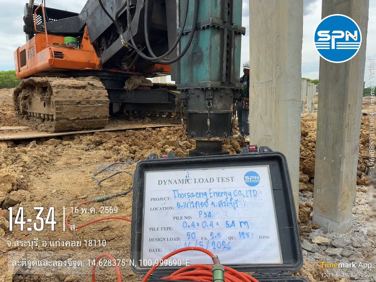
PDA equipment recording force and velocity signals at the pile head on site, before the data is analyzed with CAPWAP signal matching
The PDA records stress-wave signals at the pile head on site; this data set is the raw input for CAPWAP analysis (photo: SPN Soil Engineering)

How Does CAPWAP Work? Explained Without Equations

CAPWAP makes a computer model "mimic" the real pile as closely as possible, then reads the capacity from that model. There are four main steps:

Force and velocity graphs measured at the pile head during driving in a PDA test — the raw data input into CAPWAP analysis
Raw field data: force (solid line) and velocity (dashed line) signals at the pile head from one blow — the raw input for CAPWAP (actual analysis result: SPN Soil Engineering)
  1. Record real signals on site — sensors at the pile head measure force and velocity over the whole period the wave travels down and reflects back, from one blow selected for analysis
  2. Build the pile–soil model — the pile is divided into connected segments; the soil along the shaft and beneath the toe is represented by springs (static resistance) and dampers (dynamic resistance)
  3. Signal matching — part of the signal is input into the model, and the other part predicted by the model is compared with the measured one. Soil parameters are adjusted repeatedly until the discrepancy (match quality) is minimized
  4. Read results from the matched model — once the model reproduces the real pile, the static resistance in the model is the estimate of the real pile's bearing capacity

Each soil element in the model is defined by three values: the maximum static resistance of that element; quake, the pile movement needed before resistance reaches its maximum; and damping, the resistance that increases with pile velocity. These three values are what the engineer adjusts during signal matching.

The figure below combines the four steps into one loop. Follow the orange arrows cycling between steps ② and ③, which repeat until the computed force overlays the measured force. The right-hand panel compares the Case Method with CAPWAP.

Diagram of the CAPWAP signal-matching loop, from measured PDA signals, the pile–soil model and force comparison with repeated soil adjustment to the final result, with a table comparing the Case Method and CAPWAP Process diagram with two panels and a bottom strip. The left panel is the CAPWAP signal-matching loop; numbers one to four match the four steps in the article. Step one: measured signals from the PDA at the pile head, split into a velocity card, which is input into the model, and a force card, which serves as the comparison target. Step two: the pile–soil model; the pile is divided into six segments, each with a green bar for the static soil resistance around that segment, the bars growing longer with depth, plus a blue bar for the toe resistance. Every segment and the toe also have quake and damping values. The model computes a force and passes it down to step three. Step three: signal matching; a graph compares the measured force as a solid navy line with the computed force as a dashed orange line, and the gap between the two lines, shaded light red, is the match quality. If they do not yet match, an orange arrow leads to the soil adjustment box on the right, which has three sliders for static resistance, quake and damping, then loops back into the model for recalculation, repeating until the gap is minimized. Once matched, a green arrow leads down to the bottom strip. Step four: read results from the matched model, namely the total capacity RU at that blow, the split between skin friction SF and end bearing EB, the distribution of resistance with depth for comparison with soil boring results, and a simulated load–settlement curve equivalent to a static load test. The right panel is a five-item comparison table of the Case Method and CAPWAP. The Case Method is computed by the PDA on site, gives results immediately after every blow, assumes a single damping value for the whole system, cannot separate skin and toe resistance, and is used for real-time site control. CAPWAP is analyzed by an engineer in the office, gives results after analysis, usually within a few days, adjusts soil values segment by segment until the signals match, separates skin and toe resistance, and is the official PDA result report. All curves are conceptual examples, not measured signals. How CAPWAP works: the signal-matching loop Not to scale 4 steps: measure → model → compare → read Repeat ② ↔ ③ until computed force overlays measured 1 Measured signals From PDA at pile head Velocity (v) Input to model Force (F) Comparison target 2 Pile–soil model Static resist. Every segment + Quake + Damping Pile toe Computed force 3 Signal matching Meas. Calc. Gap = Match Quality No match Adjust soil Static resist. Quake Damping Repeat Matched → read Curves: conceptual examples Case Method vs CAPWAP Field value vs. detailed analysis Case Method CAPWAP Where On site Computed by PDA Office Engineer analysis When Instant Every blow After analysis Usually a few days Soil parameters Assumed damping One for system Per segment Until match Skin / toe split No Yes Role Site control Real time Official report of PDA results Summary of the comparison table in the article 4 Read results from the matched model Total capacity RU at that blow Skin / toe split SF and EB Resist. vs. depth Vs. boring results Load–Settlement Like static test
CAPWAP signal-matching loop — ① velocity and force signals measured by the PDA; ② pile model divided into segments, each with static resistance, quake and damping; ③ computed force compared with measured force, and if they do not match, soil values are adjusted and the loop repeats; ④ results read once the signals match. The right-hand panel summarizes the differences between the Case Method and CAPWAP (curves are conceptual examples, not measured signals · figure: SPN Soil Engineering)

When the loop ends, the actual result looks like the next figure: the measured force curve and the model-computed curve overlap almost perfectly.

CAPWAP signal-matching graph comparing measured force (Force Msd) with model force (Force Cpt), which overlap almost perfectly
Signal matching result: the measured force (Force Msd — solid line) and the model-predicted force (Force Cpt — dashed line) overlap almost perfectly, showing that the model reproduces the real pile well, so the capacity read from the model is reliable

What Results Does CAPWAP Provide?

CAPWAP provides five results from a single blow: total capacity, the split between skin and toe resistance, the distribution of resistance with depth, a simulated load–settlement curve, and the maximum stress in the pile during driving. The table below summarizes what each value tells you and how it is used.

← Scroll to see the full table →

ResultWhat it tells youWhat it is used for
Total capacityTotal static resistance of the pile at that blowCompare with the design capacity
Skin friction / end bearing splitHow much resistance comes from the shaft and how much from the toeCheck whether the pile behaves as designed
Skin friction distribution with depthWhich soil layers provide more or less resistanceCompare with soil boring results to confirm the toe has reached the bearing layer
Simulated load–settlement curveSettlement behavior equivalent to a static load testEstimate settlement at working load without a static test on every pile
Maximum stress in the pile during drivingWhether the pile is at risk of driving damageControl driving energy to keep the pile safe

Example from an actual analysis: a pile with a cross-section of 1,225 cm² embedded about 26 m deep. The CAPWAP result gave a total capacity (RU) of 194 t, split into 164 t of skin friction (SF) and 30 t of end bearing (EB). About 85% of the resistance comes from the shaft, so this pile behaves as a friction pile — information a single on-site value cannot provide.

Shaft resistance distribution graph and pile force at RU from a CAPWAP analysis, showing the proportions of skin friction and end bearing
Skin friction distribution with depth: the bars at the top show that the lower soil provides more friction with depth, while the curve below shows the force in the pile decreasing from the pile head (194 t) to just EB 30 t at the toe
Simulated load–settlement curve from a CAPWAP result, showing the relationship between applied load and settlement at the pile head and toe, with a total capacity of 194 t
Simulated load–settlement curve equivalent to a static load test: load increases to RU 194 t at a settlement of about 10.5 mm (Dy), with a permanent set from this blow of 2 mm/blow

A real-world example: a pile designed to carry load mainly in end bearing, but whose CAPWAP result shows almost all resistance coming from the shaft, is a signal that the engineer must verify whether the toe has actually reached the bearing layer. See how to read the other values in the article Reading PDA test results

The SF, EB and RU values above are read from the same model. The 3D view below opens up its interior: the sum of the green springs along the shaft is SF, the blue spring at the toe is EB, and the right-hand panel summarizes the limitations you need to know before reading the results.

Conceptual 3D model showing the inside of a CAPWAP model, with the pile divided into segments, each having springs and dampers representing the surrounding soil, and springs and dampers at the toe representing the soil beneath it, plus a summary of the values read and the limitations Conceptual 3D view of a soil block with its front corner cut away to show the inside. The soil wall is divided into three layers: soft clay at the top, stiff clay in the middle and sand at the bottom. A solid square pile stands in the cut-out, separated into five segments with small gaps to show that the model divides the pile into segments. An orange arrow above the pile head represents the hammer impact that sends a wave down the pile. Each segment is connected to the left soil wall by a green spring representing static resistance, and to the right soil wall by a navy damper representing dynamic resistance, or damping. In the actual model every segment has both; they are drawn on opposite sides for clarity. Beneath the toe, a blue spring and damper connect down to a base plate in the sand layer, representing the soil beneath the toe. A small box at the lower left explains that each soil element is defined by three values: a graph of static resistance versus pile movement that rises linearly up to the quake distance and then stays constant at the maximum static resistance, and damping, which makes resistance increase with pile velocity. The right-hand panel summarizes how values are read: the sum of the shaft springs is the skin friction SF, the toe spring is the end bearing EB, and SF plus EB equals the total capacity RU. The article's example is SF 164 t plus EB 30 t equals RU 194 t, with about 85 percent from the shaft, so it behaves as a friction pile. This is followed by four limitations: the value is the capacity at the time of driving — clay shows soil setup and some dense sands may show relaxation, so restrike testing is required per the specification; the pile must move enough — if the set is very small, the value is only a lower bound; the signals must be good and the report should show match quality; and the analyst must understand both wave theory and soil behavior. This is a conceptual image, not to scale. 3D model: inside the CAPWAP model Not to scale Hammer impact Wave travels down pile Force & velocity gauges Data input to model Pile segments Split to show joints Spring ① Static resist. ② Quake Damper ③ Damping Soft clay Stiff clay Sand Soil below toe Spring + damper Each soil element = 3 adjustable values ① ② Quake Force → Disp. → ① Static resist. Max. that soil can resist ② Quake Movement to reach max. ③ Damping Faster pile, more resistance Reading the model Sum of shaft springs = skin friction (SF) Toe spring = end bearing (EB) SF + EB = RU (total) Article example SF 164 + EB 30 = RU 194 t About 85% from shaft → friction pile behavior Key limitations 1 Capacity at driving time Clay set-up · sand relaxation → restrike testing 2 Pile must move enough Very small set = lower bound only 3 Signals must be good Report should show Match Quality 4 The analyst matters Must know waves and soil A good spec states values from End of Drive or Restrike Conceptual view · Not to scale
Inside the CAPWAP model (exploded view) — the pile is divided into segments, each with a spring (static resistance + quake) and a damper (damping) representing the surrounding soil. In the actual model every segment has both; they are drawn on opposite sides for clarity. The toe has a spring and damper representing the soil beneath it. The figures in the right-hand panel come from the example in this article (conceptual image, not to scale · figure: SPN Soil Engineering)

What to Watch for When Reading CAPWAP Results

CAPWAP results are reliable when the signals are good, the pile moves enough, and the reader understands that the value is the capacity at the time of driving. There are five things to know.

  • The value is the capacity at the time of driving — piles driven in clay show soil setup, meaning capacity increases with time after driving. Results from end-of-drive blows are therefore usually lower than those from re-driving after a waiting period (restrike test). Conversely, dense sand or some shales may show relaxation, meaning capacity decreases after driving. A good specification therefore states which blows the values should be taken from. For more on test timing, see How long to wait before testing piles
  • Match quality matters — a good report should show the match quality value and a graph comparing measured and modeled signals, so the reliability of the analysis can be checked
  • The pile must move enough — if the pile barely moves under the blow (very small set per blow), the soil resistance may not be fully mobilized, and the analyzed value will only be a lower bound of the true capacity
  • The analyst affects quality — signal matching requires an engineer who understands both wave theory and soil behavior, not just pressing a button to let the software run automatically
  • Check against the criteria of the Foundation Ministerial Regulation B.E. 2566 (2023) — the analyzed capacity must be at least 2.5 times the design working load (FS = 2.5). Acceptance is the responsibility of the design engineer according to the project requirements. See all eight key values and a detailed report interpretation example in How to Read PDA Test Results — A Guide to Dynamic Load Test Analysis

How Does CAPWAP Differ from the Case Method and a Static Load Test?

The Case Method is the fastest but gives a preliminary estimate. CAPWAP is detailed and can separate skin and toe resistance. A static load test is the most direct measurement but takes the most time and budget. A conventional static load test cannot separate skin and toe resistance; that requires an instrumented pile.

← Scroll to see the full table →

TopicCase Method (on site)CAPWAP (detailed analysis)Static Load Test
Speed of resultsImmediately after every blowAfter analysis (usually within a few days)Several days to weeks
ResolutionPreliminary estimateHigh; separates force componentsHighest (direct measurement)
Friction / end bearing splitNoYesNot directly (requires additional instrumentation in the pile)
Role in the projectReal-time site controlOfficial PDA result reportReference test / calibration
📋 How the three methods relate

The Case Method supports real-time decisions on site → CAPWAP is the official analysis that should be in every PDA report → a static load test is the ultimate calibration when the project requires it

SPN Soil Engineering provides complete pile testing services, including dynamic load testing (PDA) with CAPWAP analysis, seismic integrity testing and static load testing to ASTM and DPT standards, with more than 20 years of experience across Thailand. Reports are certified by a civil engineer licensed by the Council of Engineers Thailand (COE) and can be submitted to the relevant authorities for building permits.